Pandarus
Pandarus is a GIS software toolkit for regionalized life cycle assessment (LCA). It is designed to work with brightway LCA framework, brightway2-regional, and Constructive Geometries. A separate library, pandarus-remote, provides a web API to run Pandarus on a server.
In the context of life cycle assessment, regionalization means the introduction of detailed spatial information for inventory activities and impact assessment characterization maps. As these will have different spatial scales, GIS functionality is required to overlay these two maps. Pandarus can do the following:
- Overlay two vector datasets, calculating the areas of each combination of features using the Mollweide projection.
- Calculate the area of the geometric difference (the areas present in one input file but not in the other) of one vector dataset with another vector dataset.
- Calculate statistics such as min, mean, and max when overlaying a raster dataset with a vector dataset.
- Normalize raster datasets, including use of compatible nodata values
- Vectorization of raster datasets
The outputs from Pandarus can be used in LCA software which does not include a GIS framework, thus speeding the integration of regionalization into the broader LCA community. There is also a conference presentation video introducing Pandarus and its integration into LCA software.
Pandarus is open source under the BSD 3-clause license.
Contents
Usage example
In addition to this documentation, there is also a Jupyter notebook usage example.
Intersecting two vector datasets
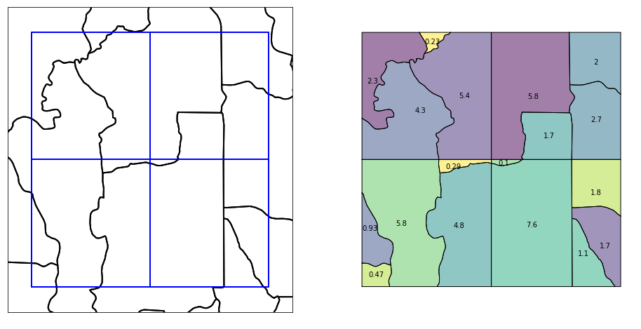
The main capability of the Pandarus library is to efficiently and correctly intersect the set of spatial features from one vector dataset with the spatial features from another vector dataset. In regionalized life cycle assessment, the first dataset would be inventory locations (polygons, lines, or points), and the second dataset would be regions with site-dependent characterization factors.
-
pandarus.intersect(first_fp, first_field, second_fp, second_field, first_kwargs={}, second_kwargs={}, dirpath=None, cpus=4, driver='GeoJSON', compress=True, log_dir=None) Calculate the intersection of two vector spatial datasets.
The first spatial input file must have only one type of geometry, i.e. points, lines, or polygons, and excluding geometry collections. Any of the following are allowed: Point, MultiPoint, LineString, LinearRing, MultiLineString, Polygon, MultiPolygon.
The second spatial input file must have either Polygons or MultiPolygons. Although no checks are made, this and other functions make a strong assumption that the spatial units in the second spatial unit do not overlap.
Input parameters:
first_fp: String. File path to the first spatial dataset.first_field: String. Name of field that uniquely identifies features in the first spatial dataset.second_fp: String. File path to the second spatial dataset.second_field: String. Name of field that uniquely identifies features in the second spatial dataset.first_kwargs: Dictionary, optional. Additional arguments, such as layer name, passed to fiona when opening the first spatial dataset.second_kwargs: Dictionary, optional. Additional arguments, such as layer name, passed to fiona when opening the second spatial dataset.dirpath: String, optional. Directory to save output files.cpus: Integer, default ismultiprocessing.cpu_count(). Number of CPU cores to use when calculating. Usecpus=0to avoid starting a multiprocessing pool.driver: String, default isGeoJSON. Fiona driver name to use when writing geospatial output file. Common values areGeoJSONorGPKG.compress: Boolean, default is True. Compress JSON output file.log_dir: String, optional.
Returns filepaths for two created files.
The first is a geospatial file that has the geometry of each possible intersection of spatial units from the two input files. The geometry type of this file will depend on the geometry type of the first input file, but will always be a multi geometry, i.e. one of MultiPoint, MultiLineString, MultiPolygon. This file will also always have the WGS 84 CRS. The output file has the following schema:
id: Integer. Auto-increment field starting from zero.from_label: String. The value for the uniquely identifying field from the first input file.to_label: String. The value for the uniquely identifying field from the second input file.measure: Float. A measure of the intersected shape. For polygons, this is the area of the feature in square meters. For lines, this is the length in meters. For points, this is the number of points. Area and length calculations are made using the Mollweide projection.
The second file is an extract of some of the feature fields in the JSON data format. This is used by programs that don’t need to depend on GIS data libraries. The JSON format is:
{
    'metadata': {
        'first': {
            'field': 'name of uniquely identifying field',
            'path': 'path to first input file',
            'filename': 'name of first input file',
            'sha256': 'sha256 hash of input file'
        },
        'second': {
            'field': 'name of uniquely identifying field',
            'path': 'path to second input file',
            'filename': 'name of second input file',
            'sha256': 'sha256 hash of input file'
        },
        'when': 'datetime this calculation finished, ISO format'
    },
    'data': [
        [
            'identifying field for first file',
            'identifying field for second file',
            'measure value'
        ]
    ]
}
Calculating areas
Because Pandarus was designed for global data sets, the Mollweide projection is used as the default equal-area projection for calculating areas (in square meters). Although no projection is perfect, the Mollweide has been found to be a reasonable compromise [1].
| [1] | Usery, E.L., and Seong, J.C., (2000) A comparison of equal-area map projections for regional and global raster data |
Projections through the calculation chain
The function intersect calls intersection_dispatcher, which in turns calls intersection_worker, which itself calls get_intersection.
In both intersect and intersection_dispatcher, spatial units from both the first and second datasets are unprojected. Inside the function intersection_worker, spatial units from the first dataset are projected to WGS 84. get_intersection calls Map.iter_latlong on the second dataset, which returns spatial units projected in WGS 84. Area and linear calculations are done on the intersection of spatial units from both the first and second spatial datasets, and are projected to the Mollweide CRS. This projection is done at the time of areal or length calculations.
Lines and points that intersect two vector features
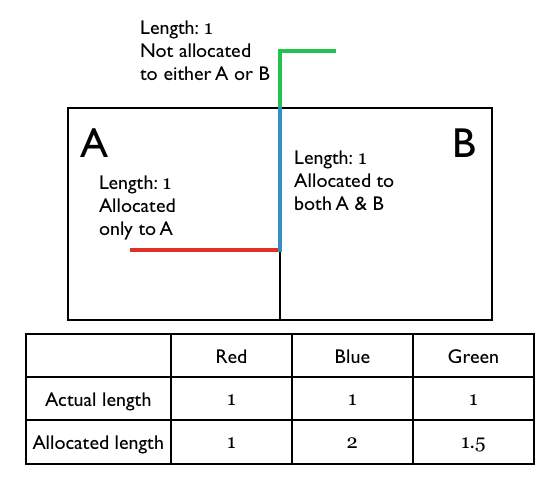
When calculating the lengths of lines (or number of points) remaining outside a intersected areas, we have the problem that lines can lie along the edge of two vector features, and hence the section of the line would be counted twice. If therefore need to adjust our formula for calculating the lengths (or number of points) outside an intersected area. The key insight is that we don’t want the actual remaining area, but the right relative remaining area - these value are all normalized to one anyway.
The formula for allocating lengths is therefore:
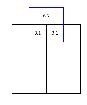
In the example above, the formula would give the answer 1.5:
The same procedure is followed for multipoints (geometries that have more than one point), except that instead of calculating lengths you just count the number of points.
Calculating area outside of intersections
For many regionalized methodologies, it is important to know how much area/length from one spatial dataset lies outside a second spatial dataset entirely. The function calculate_remaining calculates these remaining areas.
-
pandarus.calculate_remaining(source_fp, source_field, intersection_fp, source_kwargs={}, dirpath=None, compress=True) Calculate the remaining area/length/number of points left out of an intersections file generated by
intersect.Input parameters:
source_fp: String. Filepath of the input spatial data which could have features outside of the intersection result.source_field: String. Name of field that uniquely identifies features in the input spatial dataset.intersection_fp: Filepath of the intersection spatial dataset generated by theintersectfunction.source_kwargs: Dictionary, optional. Additional arguments, such as layer name, passed to fiona when opening the input spatial dataset.dirpath: String, optional. Directory where the output file will be saved.compress: Boolean. Whether or not to compress the output file.
Warning
source_fpmust be the first file provided to theintersectfunction, not the second!Returns the filepath of the output file. The output file JSON format is:
{
    'metadata': {
        'source': {
            'field': 'name of uniquely identifying field',
            'path': 'path to the input file',
            'filename': 'name of the input file',
            'sha256': 'sha256 hash of the input file'
        },
        'intersections': {
            'field': 'name of uniquely identifying field (always `id`)',
            'path': 'path to intersections spatial dataset',
            'filename': 'name of intersections spatial dataset',
            'sha256': 'sha256 hash of intersection spatial dataset'
        }
        'when': 'datetime this calculation finished, ISO format'
    },
    'data': [
        [
            'identifying field for source file',
            'measure value'
        ]
    ]
}
Using intersections spatial dataset as a new spatial scale
-
pandarus.intersections_from_intersection(fp, metadata=None, dirpath=None) Process an intersections spatial dataset to create two intersections data files.
fpis the file path of a vector dataset created by theintersectfunction. The intersection of two spatial scales (A, B) is a third spatial scale (C); this function creates intersection data files for (A, C) and (B, C).As the intersections data file includes metadata on the input files, this function must have access to the intersections data file created at the same time as intersections spatial dataset. If the
metadatafilepath is not provided, the metadata file is looked for in the same directory asfp.Returns the file paths of the two new intersections data files.
Calculating raster statistics against a vector dataset
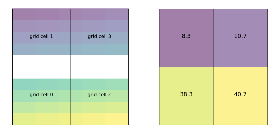
Pandarus can calculate mask a raster with each feature from a vector dataset, and calculate the min, max, and average values from the intersected raster cells. This functionality is provided by a patched version of rasterstats.
The vector and raster file should have the same coordinate reference system. No automatic projection is done by this function.
-
pandarus.raster_statistics(vector_fp, identifying_field, raster, output=None, band=1, compress=True, fiona_kwargs={}, **kwargs) Create statistics by matching
rasteragainst each spatial unit inself.from_map.For each spatial unit in
self.from_map, calculates the following statistics for values fromraster: min, mean, max, and count. Count is the number of raster cells intersecting the vector spatial unit. No data values in the raster are not including in the generated statistics.This function uses a fork of the
rasterstatslibrary that break each raster cell into 100 smaller cells, as a compromise approach to handle the fact that some raster cells are completely with a vector geometry, while others only have a small fraction of their cell area within the vector geometry. Each of the 100 small raster cells is weighted equally, and each is tested to make sure it intersects the vector geometry.This function assumes that each smaller raster cell has the same area. This may change in the future.
Input parameters:
vector_fp: str. Filepath of the vector dataset.identifying_field: str. Name of the field invector_fpthat uniquely identifies each feature.raster: str. Filepath of the raster dataset.output: str, optional. Filepath of the output file. Will be deleted if it exists already.band: int, optional. Raster band used for calculations. Default is1.compress: bool, optional. Compress JSON results file. Default isTrue.fiona_kwargs: dict, optional. Additional arguments to pass to fiona when openingvector_fp.
Any additional
kwargsare passed togen_zonal_stats.Output format:
Output is a (maybe compressed) JSON file with the following schema:
{
    'metadata': {
        'vector': {
            'field': 'name of uniquely identifying field',
            'path': 'path to vector input file',
            'sha256': 'sha256 hash of input file'
        },
        'raster': {
            'band': 'band used to calculate raster stats',
            'path': 'path to raster input file',
            'filename': 'name of raster file',
            'sha256': 'sha256 hash of input file'
        },
        'when': 'datetime this calculation finished, ISO format'
    },
    'data': [
        [
            'vector `identifying_field` value',
            {
                'count': 'number of raster cells included. float because consider fractional intersections',
                'min': 'minimum raster value in this vector feature',
                'mean': 'average raster value in this vector feature',
                'max': 'maximum raster value in this vector feature',
            }
        ]
    ]
}
Manipulating raster files
Pandarus provides some utility functions to help manage and manipulate raster files. Raster files are often provided with incorrect or missing metadata, and the main pandarus capabilities only work on vector files. Unfortunately, however, many raster files require manual fixes outside of these functions.
-
pandarus.clean_raster(fp, new_fp=None, band=1, nodata=None) - Clean raster data and metadata:
- Delete invalid block sizes, and remove tiling
- Set nodata to a reasonable value, if possible
- Convert to 32 bit floats, if currently 64 bit floats and such conversion is possible
fp: String. Filepath of the input raster file.new_fp: String, optional. Filepath of the raster to create. If not provided, the new raster will have the same name as the existing file, but will be created in a temporary directory.band: Integer, default is1. Raster band to clean and create in new file. Each band of a multiband raster would have to be cleaned separately.nodata: Float, optional. Additional value to try when changingnodatavalue; must not be present in existing raster data.Returns the filepath of the new file as a compressed GeoTIFF. Can also return
Noneif no new raster was written due to failing preconditions.
-
pandarus.round_raster(in_fp, out_fp=None, band=1, sig_digits=3) Round raster cell values to a certain number of significant digits in new raster file. For example, π rounded to 4 significant digits is 3.142.
in_fp: String. Filepath of raster input file.out_fp: String, optional. Filepath of new raster to be created. Should not currently exist. If not provided, the new raster will have the same name as the existing file, but will be created in a temporary directory.band: Int, default is 1. Band to round. Band indices start at 1.sig_digits: Int, default is 3. Number of significant digits to round to.
The created raster file will have the same
dtype, shape, and CRS as the input file. It will be a compressed GeoTIFF.Returns
out_fp, the filepath of the created file.
-
pandarus.convert_to_vector(filepath, dirpath=None, band=1) Convert raster file at
filepathto a vector file. Returns filepath of created vector file.dirpathshould be a writable directory. Ifdirpathis no specified, uses the appdirs library to find an appropriate directory.bandshould be the integer index of the band; default is 1. Note that band indices start from 1, not 0.The generated vector file will be in GeoJSON, and have the WGS84 CRS.
Because we are using GDAL polygonize, we can’t use 64 bit floats. This function will automatically convert rasters from 64 to 32 bit floats if necessary.
FAQ
Why the name Pandarus?
The software overlays (matches) two different maps, and Pandarus was a bit of a matchmaker himself. Plus, ancient names are 172% more science-y.
Installation
Pandarus can be installed directly from PyPi using pip or easy_install, e.g.
pip install pandarus
However, it is easy to run into errors if geospatial libraries like fiona, rasterio, and shapely are compiled against different versions of GDAL. One way to get an installation that is almost guaranteed is to use Conda:
conda create -n <virtualenv name> python=3.6
activate <virtualenv name>  # Could also be source activate <virtualenv name>
conda install -c conda-forge -c cmutel pandarus
You should replace <virtualenv name> with a name you will remember.
Pandarus is only compatible with Python >= 3.5. Source code is on GitHub.
Contributing
Contributions are welcome via pull requests and issues on Github. Please ensure that pull requests include tests and documentation. Pandarus follows the Contributor Covenant code of conduct.